Lecture 6 - Training CNN Model using MNIST Dataset#
For this demonstration we will be using MNIST dataset which is a popular dataset in training deep learning models.
Import Standard Libraries
import torch
import torch.nn as nn
import torch.nn.functional as F
from torch.utils.data import DataLoader
import torchvision
from torchvision import datasets, transforms

import random
import numpy as np
from sklearn.metrics import confusion_matrix, classification_report, accuracy_score
import matplotlib.pyplot as plt
%matplotlib inline

torch.backends.cudnn.deterministic=True
torch.set_printoptions(sci_mode=False)

import time
from tqdm.notebook import tqdm
---------------------------------------------------------------------------
ModuleNotFoundError                       Traceback (most recent call last)
Cell In[1], line 18
     15 torch.set_printoptions(sci_mode=False)
     17 import time
---> 18 from tqdm.notebook import tqdm

ModuleNotFoundError: No module named 'tqdm'
torchvision.datasets module provides a variety of datasets that are commonly used for training machine learning and deep learning models. These datasets are preprocessed and can be easily integrated into PyTorch workflows for tasks such as image classification, object detection, and more. Dataset includes:
MNIST
CIFAR10
CIFAR100
ImageNet
# `transforms` is used to apply augmentation techniques and modification to the image data (e.g, rotate, resize, normalization, etc.).
# for this one, let's just convert the image arrays to tensor.
transform = transforms.ToTensor()

train_data = datasets.MNIST(root='data', train=True, download=True, transform=transform)
test_data  = datasets.MNIST(root='data', train=False, download=True, transform=transform)
# the training data have 60,000 images, let's take a small portion from it for the validation.
# what's the importance of validation data?
train_data
Dataset MNIST
    Number of datapoints: 60000
    Root location: data
    Split: Train
    StandardTransform
Transform: ToTensor()
# unseen images
test_data
Dataset MNIST
    Number of datapoints: 10000
    Root location: data
    Split: Test
    StandardTransform
Transform: ToTensor()
# 50,000 for training and 10,000 for validation
train_set, val_set = torch.utils.data.random_split(train_data, [0.8, 0.2])
# function to set the seed
def set_seed(seed):
    np.random.seed(seed)
    torch.manual_seed(seed)
    random.seed(seed)
PyTorch provides two data primitives: torch.utils.data.DataLoader and torch.utils.data.Dataset that allow you to use pre-loaded datasets as well as your own data. Dataset stores the samples and their corresponding labels, and DataLoader wraps an iterable around the Dataset to enable easy access to the samples.
set_seed(143)

batch_size = 10

train_loader = DataLoader(train_set, batch_size=batch_size, shuffle=True)
val_loader = DataLoader(val_set, batch_size=batch_size, shuffle=True)
test_loader = DataLoader(test_data, batch_size=batch_size, shuffle=False)
set_seed(143)
images, labels = iter(train_loader).__next__()

def display_image(batch):
    batch = batch.detach().numpy()
    fig, axs = plt.subplots(1, len(batch), figsize=(12, 2))
    for i in range(len(batch)):
        axs[i].imshow(batch[i, 0, :, :], vmin=0, vmax=1)
        axs[i].axis('off')
        axs[i].set_title(labels[i].numpy())
    plt.show()
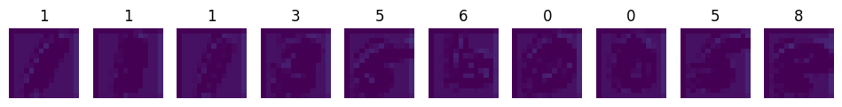
For this demonstration, we will use the following architecture: it consists of two convolutional layers, each followed by its own max-pooling layer and activation function. Additionally, there are two fully connected layers, with the second layer using the softmax activation function.
Input Images
display_image(images)
print(images.shape)

# (b, c, h, w)
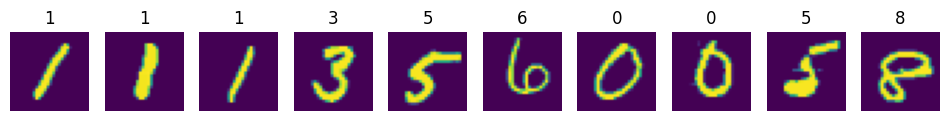
torch.Size([10, 1, 28, 28])
def calc_out(w, f, s, p):
    """
    Calculate output shape of a matrix after a convolution.
    The results are only applicable for square matrix kernels and images only.
    """
    print(f'Output Shape: {(w - f + 2 * p) // s + 1}')
First Convolution Layer + Activation Function
# The first convolution must output a 28 by 28 image size
calc_out(28, 3, 1, 1)
Output Shape: 28
conv1 = nn.Conv2d(1, 32, (3,3), 1, 1)

x = F.relu(conv1(images))
display_image(x)
print(x.shape)
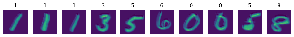
torch.Size([10, 32, 28, 28])
First Pooling (MaxPooling)
# first maxpooling must output a 14 by 14 size
calc_out(28, 2, 2, 0)
Output Shape: 14
pool1 = nn.MaxPool2d((2,2), 2)

x = pool1(x)
display_image(x)
print(x.shape)
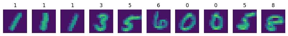
torch.Size([10, 32, 14, 14])
Let’s examine the feature map.
idx = 3
feature_maps =  x[idx].view((1, 32, 14, 14)).detach().numpy()
fig, axs = plt.subplots(1, 32, figsize=(12, 2))
for i in range(32):
    axs[i].imshow(feature_maps[0, i, :, :], vmin=0, vmax=1)
    axs[i].axis('off')
Second Convolution
calc_out(14, 3, 1, 1)
Output Shape: 14
conv2 = nn.Conv2d(32, 64, (3,3), 1, 1)

x = F.relu(conv2(x))
display_image(x)
print(x.shape)

torch.Size([10, 64, 14, 14])
Second Pooling (MaxPooling)
calc_out(14, 2, 2, 0)
Output Shape: 7
pool2 = nn.MaxPool2d((2,2), 2)

x = pool2(x)
display_image(x)
print(x.shape)
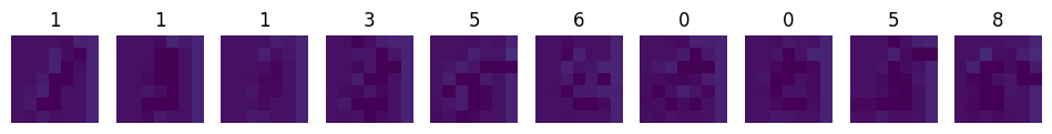
torch.Size([10, 64, 7, 7])
idx = 3
feature_maps =  x[idx].view((1, 64, 7, 7)).detach().numpy()
fig, axs = plt.subplots(1, 64, figsize=(12, 2))
for i in range(64):
    axs[i].imshow(feature_maps[0, i, :, :], vmin=0, vmax=1)
    axs[i].axis('off')
Flatten
flat = x.view((-1, 64*7*7))

fcn1 = nn.Linear(64*7*7, 128)
fcn2 = nn.Linear(128, 10)

out = fcn1(flat)
out = F.softmax(fcn2(out), dim=1)
# prediction
# assess the prediction
[i.argmax().item() for i in out]
[4, 8, 8, 4, 4, 4, 4, 4, 4, 4]
# true label
[i.item() for i in labels]
[1, 1, 1, 3, 5, 6, 0, 0, 5, 8]
QUESTION:
Why is it that the true and the predicted value is very distant from each other?
Now let’s put them all together
class CNN(nn.Module):
    def __init__(self):
        super().__init__()
        # just the initialization
        self.conv1 = nn.Conv2d(1, 32, (3,3), 1, 1)
        self.pool1 = nn.MaxPool2d((2,2), 2)
        self.conv2 = nn.Conv2d(32, 64, (3,3), 1, 1)
        self.pool2 = nn.MaxPool2d((2,2), 2)
        self.fcn1 = nn.Linear(64*7*7, 128)
        self.fcn2 = nn.Linear(128, 10)

    def forward(self, x):
        # seuential
        x = F.relu(self.conv1(x))
        x = self.pool1(x)
        x = F.relu(self.conv2(x))
        x = self.pool2(x)
        x = x.view(-1, 64*7*7)
        x = self.fcn1(x)
        x = F.softmax(self.fcn2(x), dim=1)

        return x
Instantiate the Class
model = CNN()
model
CNN(
  (conv1): Conv2d(1, 32, kernel_size=(3, 3), stride=(1, 1), padding=(1, 1))
  (pool1): MaxPool2d(kernel_size=(2, 2), stride=2, padding=0, dilation=1, ceil_mode=False)
  (conv2): Conv2d(32, 64, kernel_size=(3, 3), stride=(1, 1), padding=(1, 1))
  (pool2): MaxPool2d(kernel_size=(2, 2), stride=2, padding=0, dilation=1, ceil_mode=False)
  (fcn1): Linear(in_features=3136, out_features=128, bias=True)
  (fcn2): Linear(in_features=128, out_features=10, bias=True)
)
Model Parameters:#
$$ \begin{align*} & (1 \times 32 \times 3 \times 3) + 32 \ & + (32 \times 64 \times 3 \times 3) + 64 \ & + (3136 \times 128) + 128 \ & + (128 \times 10) + 10 \ & = 288 + 32 + 18432 + 64 + 401408 + 128 + 1280 + 10 \ & = 421,642 \end{align*}
def count_parameters(model):
    params = [p.numel() for p in model.parameters() if p.requires_grad]
    for item in params:
        print(f'{item:>6}')
    print(f'______\n{sum(params):>6}')

count_parameters(model)
   288
    32
 18432
    64
401408
   128
  1280
    10
______
421642
Define Criterion and Optimizer
criterion = nn.CrossEntropyLoss()
optimizer = torch.optim.Adam(model.parameters(), lr=0.001)
# if your device has cuda enabled gpu, you can use it to accelerate the training process.
device = torch.device('cuda' if torch.cuda.is_available() else 'cpu')

print(device)

model = model.to(device)
cpu
next(model.parameters()).device
device(type='cpu')
Let’s walk through the training loop
for e in range(epochs): train_corr = 0 val_corr = 0
This will iterate 5 times as what is defined below. train_corr and val_corr serves as temporary place holders for correctly predicted train data and correctly predicted validation data. Hence, train_corr and val_corr will be re-initialized to 0 again if an entire epoch is done.
for train_b, (x_train, y_train) in tqdm(enumerate(train_loader)):
    train_b += 1
    x_train = x_train.to(device)
    y_train = y_train.to(device)
for train_b, (x_train, y_train) in tqdm(enumerate(train_loader)):
    train_b += 1
    x_train = x_train.to(device)
    y_train = y_train.to(device)
The second loop (nested loop) iterates over the train_loader. A single iteration of the train_loader is equal to 1 batch of features and targets, our batch size is 10, therefore in every iteration of the train_loader we are processing 10 instances. The entire training set or the len(train_loader.dataset) is 50,000. Therefore, to finish an entire epoch, we need to process 5000 batches with a batch size of 10 (5000 x 10 = 50,000).
NOTE: When an iterable object is wrapped around an enumerate function, the output will return an index for each iterated values. train_b is the number of batches that has been processed.
The to() functions next to the x_train and y_train are simply there to move the data into the available computing device. Remember that you need to move the model as well to the available device.
OUTPUT:
x_train.shape = torch.Size([10, 1, 28, 28])
y_train.shape = torch.Size([10])
    train_pred = model(x_train)
    train_loss = criterion(train_pred, y_train)

    train_pred_vec = torch.max(train_pred.data, 1)[1]
    train_corr += (train_pred_vec == y_train).sum()
train_pred represents the model’s predictions for the current batch. The shape of train_pred is torch.Size([10, 10]). Each row in train_pred corresponds to an instance in the batch, and each column represents a class. The values in each row indicate the model’s estimated probabilities or scores for each class for that instance.
train_loss is a scalar value of the error that was calculated from that particular batch.
train_pred_vec is a vector that contained the predicted labels of the current batch. The values are integer that ranges from 0 to 9. train_pred_vec.shape is torch.Size([10]), the values represents each predicted label of each instance.
train_corr performs comparison operation to check how many samples in the batch was correctly predicted, the value of the train_corr will be inceremented, but will be re-initialized back to 0 when an entire epoch is done.
    # Update parameters
    optimizer.zero_grad()
    train_loss.backward()
    optimizer.step()
We need to update the parameters for every batch that passes in every epoch, we can do this by applying zero_grad() to the optimizer, this will clear the gradients for the next batch, if we don’t do that, the gradients will accumulate for every batch for the entire epoch.
train_loss.backward() is used to compute the gradients of the loss with respect to the model’s parameters during the backward pass of the training process. It’s a fundamental step in the training loop of a neural network.
optimizer.step() is a method used to update the parameters (weights and biases) of a neural network model during the training process. It is called after the gradients of the model’s parameters have been computed during the backward pass.
    if train_b % 1250 == 0:
        print(f"epoch: {e+1:2} | batch: {train_b:4} | instances: [{train_b*batch_size:6} / {len(train_loader)  * batch_size}] | loss: {train_loss.item()}")
        print(f"✅{train_corr.item()} of {train_b*batch_size:2} | accuracy: {round(((train_corr.item() / (train_b*batch_size))) * 100 , 3)}%")
This prints training progress information during each batch iteration in a concise format. It displays the current epoch, batch number, the number of processed instances, the loss, and the accuracy achieved up to that point in training.
    train_correct.append(train_corr.item())
    train_losses.append(train_loss.item())
Appends current the batch’s train_corr and train_loss on the empty lists outside the epoch.
with torch.no_grad():
    for val_b, (x_val, y_val) in enumerate(val_loader):
        val_b += 1

        x_val = x_val.to(device)
        y_val = y_val.to(device)

        val_pred = model(x_val)
        val_pred_vec = torch.max(val_pred.data, 1)[1]
        val_corr += (val_pred_vec == y_val).sum()

        val_loss = criterion(val_pred, y_val)
        val_correct.append(val_corr.item())
        val_losses.append(val_loss.item())

        val_acc = val_corr.item() / (len(val_loader) * batch_size)

    if val_acc > best_acc:
        best_acc = val_acc
        torch.save(model.state_dict(), f"model/best_{model._get_name()}.pth")
        print(f"\t📁New best model saved! | accuracy: {best_acc*100}%")

train_epoch_acc = train_corr.item() / (batch_size * len(train_loader))
val_epoch_acc = val_corr.item() / (batch_size * len(val_loader))

train_accs.append(train_epoch_acc)
val_accs.append(val_epoch_acc)
print(f’\nDuration: {time.time() - start_time:.0f} seconds’)
This part of the code performs the evaluation of the trained model for every epoch, the code is quite similar to the training process but without the updating of parameters. The code also have features of saving the state_dict (trained parameters) of the model with best accuracy.
import os

set_seed(42)
epochs = 5
start_time = time.time()
best_acc = 0.0

# ensure model directory exists
os.makedirs("model", exist_ok=True)

train_correct = []
train_losses = []
train_accs = []

val_correct = []
val_losses = []
val_accs = []

for e in range(epochs):
    train_corr = 0
    val_corr = 0

    for train_b, (x_train, y_train) in tqdm(enumerate(train_loader)):
        train_b += 1
        x_train = x_train.to(device)
        y_train = y_train.to(device)

        train_pred = model(x_train)
        train_loss = criterion(train_pred, y_train)

        train_pred_vec = torch.max(train_pred.data, 1)[1] # prediction vector
        train_corr += (train_pred_vec == y_train).sum()

        # Update parameters
        optimizer.zero_grad()
        train_loss.backward()
        optimizer.step()

        if train_b % 1250 == 0:
            print(f"epoch: {e+1:2} | batch: {train_b:4} | instances: [{train_b*batch_size:6} / {len(train_loader)  * batch_size}] | loss: {train_loss.item()}")
            print(f"✅{train_corr.item()} of {train_b*batch_size:2} | accuracy: {round(((train_corr.item() / (train_b*batch_size))) * 100 , 3)}%")

        train_correct.append(train_corr.item())
        train_losses.append(train_loss.item())

    with torch.no_grad():
        for val_b, (x_val, y_val) in enumerate(val_loader):
            val_b += 1

            x_val = x_val.to(device)
            y_val = y_val.to(device)

            val_pred = model(x_val)
            val_pred_vec = torch.max(val_pred.data, 1)[1]
            val_corr += (val_pred_vec == y_val).sum()

            val_loss = criterion(val_pred, y_val)
            val_correct.append(val_corr.item())
            val_losses.append(val_loss.item())

            val_acc = val_corr.item() / (len(val_loader) * batch_size)

        if val_acc > best_acc:
            best_acc = val_acc
            # directory was created at start, so this will succeed
            torch.save(model.state_dict(), f"model/best_{model._get_name()}.pth")
            print(f"\t📁New best model saved! | accuracy: {best_acc*100}%")

    train_epoch_acc = train_corr.item() / (batch_size * len(train_loader))
    val_epoch_acc = val_corr.item() / (batch_size * len(val_loader))

    train_accs.append(train_epoch_acc)
    val_accs.append(val_epoch_acc)

print(f'\nDuration: {time.time() - start_time:.0f} seconds')
epoch:  1 | batch: 1250 | instances: [ 12500 / 48000] | loss: 1.4611501693725586
✅12146 of 12500 | accuracy: 97.168%
epoch:  1 | batch: 2500 | instances: [ 25000 / 48000] | loss: 1.490952730178833
✅24304 of 25000 | accuracy: 97.216%
epoch:  1 | batch: 3750 | instances: [ 37500 / 48000] | loss: 1.4611501693725586
✅36467 of 37500 | accuracy: 97.245%
	📁New best model saved! | accuracy: 96.325%
epoch:  2 | batch: 1250 | instances: [ 12500 / 48000] | loss: 1.5611469745635986
✅12200 of 12500 | accuracy: 97.6%
epoch:  2 | batch: 2500 | instances: [ 25000 / 48000] | loss: 1.5611501932144165
✅24347 of 25000 | accuracy: 97.388%
epoch:  2 | batch: 3750 | instances: [ 37500 / 48000] | loss: 1.5611501932144165
✅36506 of 37500 | accuracy: 97.349%
	📁New best model saved! | accuracy: 97.46666666666667%
epoch:  3 | batch: 1250 | instances: [ 12500 / 48000] | loss: 1.4611501693725586
✅12242 of 12500 | accuracy: 97.936%
epoch:  3 | batch: 2500 | instances: [ 25000 / 48000] | loss: 1.5496798753738403
✅24426 of 25000 | accuracy: 97.704%
epoch:  3 | batch: 3750 | instances: [ 37500 / 48000] | loss: 1.4611501693725586
✅36625 of 37500 | accuracy: 97.667%
epoch:  4 | batch: 1250 | instances: [ 12500 / 48000] | loss: 1.5611494779586792
✅12169 of 12500 | accuracy: 97.352%
epoch:  4 | batch: 2500 | instances: [ 25000 / 48000] | loss: 1.4611501693725586
✅24293 of 25000 | accuracy: 97.172%
epoch:  4 | batch: 3750 | instances: [ 37500 / 48000] | loss: 1.4611501693725586
✅36439 of 37500 | accuracy: 97.171%
epoch:  5 | batch: 1250 | instances: [ 12500 / 48000] | loss: 1.559799075126648
✅12220 of 12500 | accuracy: 97.76%
epoch:  5 | batch: 2500 | instances: [ 25000 / 48000] | loss: 1.4611501693725586
✅24406 of 25000 | accuracy: 97.624%
epoch:  5 | batch: 3750 | instances: [ 37500 / 48000] | loss: 1.4611501693725586
✅36593 of 37500 | accuracy: 97.581%

Duration: 395 seconds
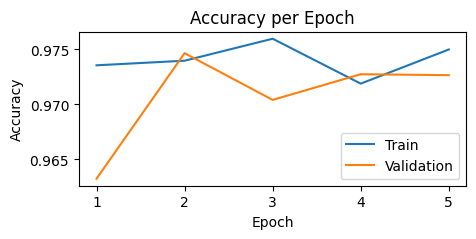
plt.figure(figsize=(5,2))
plt.plot(train_accs, label="Train")
plt.plot(val_accs, label="Validation")
plt.xticks(ticks=range(0,5), labels=list(range(1,6)))
plt.xlabel("Epoch")
plt.ylabel("Accuracy")
plt.title("Accuracy per Epoch")
plt.legend()
plt.show()

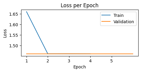
plt.figure(figsize=(5,2))
plt.plot([train_losses[i-1] for i in range(5000, len(train_losses)+1, 5000)], label="Train")
plt.plot([val_losses[i-1] for i in range(1000, len(val_losses)+1, 1000)], label="Validation")
plt.xticks(ticks=range(0,5), labels=list(range(1,6)))
plt.xlabel("Epoch")
plt.ylabel("Loss")
plt.title("Loss per Epoch")
plt.legend()
plt.show()
Testing
true_labels = []
pred_labels = []

with torch.no_grad():
    for b, (x_test, y_test) in enumerate(test_loader):

        x_test = x_test.to(device)
        y_test = y_test.to(device)

        test_pred = model(x_test)
        test_pred_vec = torch.max(test_pred.data, 1)[1]

        true_labels.append(y_test)
        pred_labels.append(test_pred_vec)
true_labels = torch.cat(true_labels, dim=0)
pred_labels = torch.cat(pred_labels, dim=0)
Classification Matrix
[v for k,v in train_data.class_to_idx.items()]
[0, 1, 2, 3, 4, 5, 6, 7, 8, 9]
true_labels
tensor([7, 2, 1, ..., 4, 5, 6])
pred_labels
tensor([7, 2, 1, ..., 4, 5, 6])
np.set_printoptions(formatter=dict(int=lambda x: f'{x:3}'))
print(np.array([v for k,v in train_data.class_to_idx.items()]), '\n')
print(confusion_matrix(true_labels.to('cpu'), pred_labels.to('cpu')))
[  0   1   2   3   4   5   6   7   8   9]

[[969   0   0   0   0   0   9   1   1   0]
 [  0 1132   3   0   0   0   0   0   0   0]
 [  2   5 1016   0   1   0   5   2   1   0]
 [  0   0  10 982   0   2   0   9   3   4]
 [  1   3   1   0 952   0  10   1   2  12]
 [  2   3   0   3   0 872   7   2   2   1]
 [  1   2   0   0   1   3 951   0   0   0]
 [  0   8  13   0   3   0   0 992   1  11]
 [  1   3   5   0   2   1   7   1 949   5]
 [  6   5   1   0   6   3   2  10   2 974]]
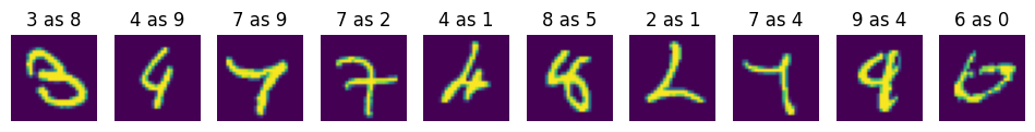
Let’s assess the misses
true_labels
tensor([7, 2, 1, ..., 4, 5, 6])
misses = np.array([])
missed_label = np.array([])

for i in range(len(pred_labels.to('cpu'))):
    if pred_labels[i] != true_labels.to('cpu')[i]:
        misses = np.append(misses,i).astype('int64')
        missed_label = np.append(missed_label, true_labels.to('cpu')[i]).astype('int64')

len(misses)
211
wrong = [pred_labels[i].item() for i in misses[:10]]
missed_images = [test_loader.dataset[j][0] for j in [i for i in misses[:10]]]
fig, axs = plt.subplots(1, len(missed_images), figsize=(12, 2))

c = 0
for i in missed_images:
    axs[c].imshow(i.view(28, 28), vmin=0, vmax=1)
    axs[c].axis('off')
    axs[c].set_title(f"{missed_label[c]} as {wrong[c]}")
    c += 1
plt.show()